Example on image classification

Example on image classification

In this section an example on real data will be presented following the lines the basic PRTools program sketched in section *. It is the intention that readers novel to PRTools just get some flavor about building and applying a recognition system. Details will be fully explained later. We will go through the program step by step. If possible, copy the lines in Matlab and look at the response in the command window or in a graphical window elsewhere on the screen.

It deals with a set of 256 color images, the Delft Image Database (delft_idb) stored in a datafile. They are organized in 9 classes named books, chess, coffee, computers, mug, phone, plant, rubbish and sugar. First it should be checked whether the data is available.

  prdatafiles

This command checks whether the so-called prdatafiles are available on your system. This is a collection of datafile examples and the Matlab commands to load the data. If needed the commands are automatically downloaded it from the PRTools website. More details are given elsewhere.

By the following statement the data itself is downloaded if needed and all details of the datafile like filenames and class labels are stored into a variable.

  A = delft_idb

and PRTools responds with a number of details about the datafile:

  Delft Image Database, raw datafile with 256 objects in 9 crisp classes: [19  44  33  35  41  30  18   9  27]

The images can be shown by:

  show(A) 

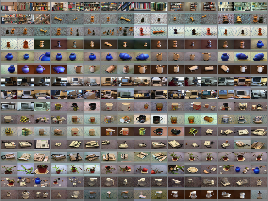
Display may take some time, especially if the datafile is stored elsewhere in the network, as all images are stored in separate files. We split the set of images at random in 80% for training (i.e. building the classification system) and 20% for testing (i.e. evaluating its performance).

  [A_train,A_test] = gendat(A,0.8) 

In this example the images will be characterized by their histograms. For real world applications much more preprocessing, like denoising and normalization on image size, intensity and contrast, may be needed. Moreover, other features than histograms may be desired. For many of them PRTools commands are available.

  W_preproc = histm([],[1:10:256]) 

By this command histograms with a bin-size of 10 are defined. As the images have three color bands (red green and blue), in total 3*26 = 78 feature values will be computed. Not that the command is just a definition of the operation. It will now be applied to the data:

  B_train = A_train*W_preproc*datasetm 

The execution of this statement takes time as all 256 images have to be processed. IF switched on a waitbar is displayed reporting the progress. Recall that in PRTools the *-operator means: 'use the variable on the left of the *-operator as input for the procedure defined on the right side of it. The routine datasetm (a PRTools mapping) converts the preprocessed datafile into a dataset, which is the PRTools construct of a collections of objects (here images) represented by vectors of the same length (here the histograms with size 78). A 78-dimensional space is too large for most classifiers to distinguish classes with at most some tens of objects. We therefore reduce the space by PCA to 8 dimensions:

  W_featred = pca(B_train,8) 

W_featred is NOT the set of objects in the reduced space, but it is the operator, trained by the PCA algorithm on the training set, that can map objects from the 78-dimensional space to the 8-dimensional space. This operator is needed explicitely as it has to be applied on the training objects as well as on all future objects to be classified.

  W_classf = fisherc(B_train*W_featred) 

Herewith the PCA mapping stored in W_featred is applied on the training set and in the reduced space the Fisher classifier is computed. This is possible as all class information of the objects is still stored, as well as in B_train as in the mapped (transformed) dataset B_train*W_featred. The total classification system is now the sequence of preprocessing, dataset conversion, feature reduction and classification. All these operations are defined in variables and the sequence can be defined by:

  W_class_sys = W_preproc*datasetm*W_featred*W_classf 

A test set can be classified by this system by

  D = A_test*W_class_sys 

All results are stored in the 256 ×9 classification matrix D. This is also a dataset. It stores class confidences or distances for all objects (256) to all classes (9). A routine labeld may be used to find for every object the most confident or nearest class by D*labeld. As D also contains the original, true labels, which may be retrieved by getlabels(D). These may be displayed together with the estimated labels:

  disp([getlabels(D) D*labeld]) 

Finally the fraction of erroneously classified objects can be found by

  D*testd 

Depending on the actual split in training and test sets the result is about 50% error. This is not very good, but it should be realized that it is a 9-class problem, and finding the correct class out of 9 in 50% of the times is still better than random. The individual classification results can be analyzed by:

  delfigs
  for i=1:47
      figure
      imagesc(imread(A_test,i))
      axis off
      truelab = getlabels(D(i,:));
      estilab = D(i,:)*labeld;
      title([truelab ' --> ' estilab])
      if ~strcmp(truelab,estilab)
          set(gcf,'Color',[0.9 0.4 0.4]);
      end
  end
  showfigs 

It might be concluded that many errors (red frames) are caused by confusing backgrounds. The backgrounds of the objects are unrelated to the objects classes. Taking histograms of the entire images is thereby not very informative.

Finally the entire example is listed for readers who want to run it in a single flow or store it for future inspection.

delfigs
  echo on

    % load the delft_idb image collection
    A = delft_idb

    % split it in a training set (80%) and a test set (20%)
    [A_train,A_test] = gendat(A,0.8)

    % define the preprocessing for the training set
    W_preproc = histm([],[1:10:256])

    % and convert it to a dataset
    B_train = A_train*W_preproc*datasetm

    % define a PCA mapping to 5 features
    W_featred = pca(B_train,8)

    % apply it to the training set and compute a classifier
    W_classf = fisherc(B_train*W_featred)

    % define the classification system
    W_class_sys = W_preproc*datasetm*W_featred*W_classf

    % classify the unlabeled testset
    D = A_test*W_class_sys

    % show the true and estimated labels
    disp([getlabels(D) D*labeld])

    % show its performance
    fprintf('Classification error: %6.3f \n',D*testd)
    input('Hit the return to continue ...');

    % show all individual test results
    delfigs
    for i=1:47
        figure
        imagesc(imread(A_test,i))
        axis off
        truelab = getlabels(D(i,:));
        estilab = D(i,:)*labeld;
        title([truelab ' --> ' estilab])
        if ~strcmp(truelab,estilab)
            set(gcf,'Color',[0.9 0.4 0.4]);
        end
    end
    showfigs

  echo off

Example on image classification