Example on silhouette classification

Example on silhouette classification

We will start with loading a simple, well known dataset of silhouettes, the Kimia dataset. It consists of a set of binary (0/1) images, representing the outlines of simple objects (e.g. toys). In the original dataset images have different sizes. The version that is used in this example has been normalized to images of 64x64 pixels.

The dataset is stored in the repository prdatasets. First it is checked whether it exists. If not, it is automatically downloaded.

    prdatasets

Now a command to load the data itself should be available and the example can be started.

    delfigs;
    a = kimia;
    show(1-a,18)

The first command, delfigs, just takes care that all existing figures (if any) are deleted.

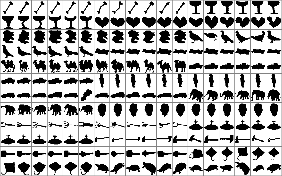
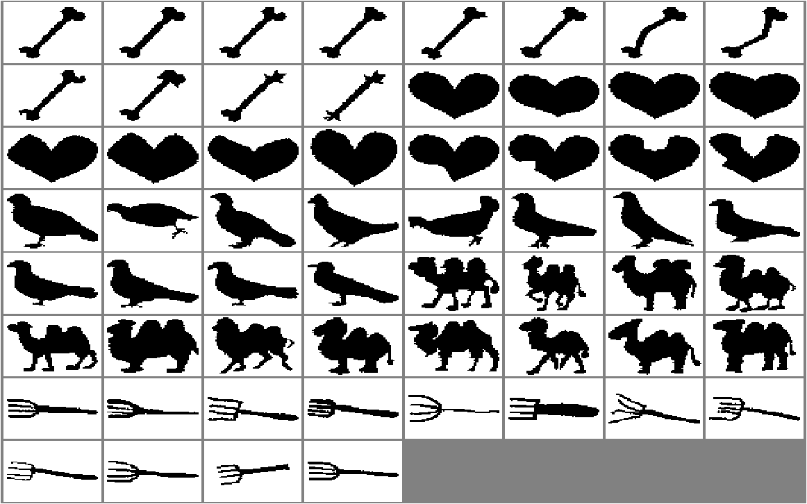
As the dataset is too large to serve as a simple illustration we will select just the classes 1, 3, 5, 7, and 13.

    b = seldat(a,[1 3 5 7,13]);
    figure; show(1-b);

Now two features (properties) will be computed for these objects: their sizes (number of pixels in an image with value 1), and the perimeter. The latter is found by two simple convolutions to compute the horizontal and vertical gradients, followed by a logical 'or' of the absolute values. The contour pixels will have a value 1 and all others are 0. The perimeter is found by a summation of all pixel values over an image.

    area = im_stat(b,'sum');
    bx = abs(filtim(b,'conv2',{[-1 1],'same'}));
    by = abs(filtim(b,'conv2',{[-1 1]','same'}));
    bor = or(bx,by);
    figure; show(1-bor);

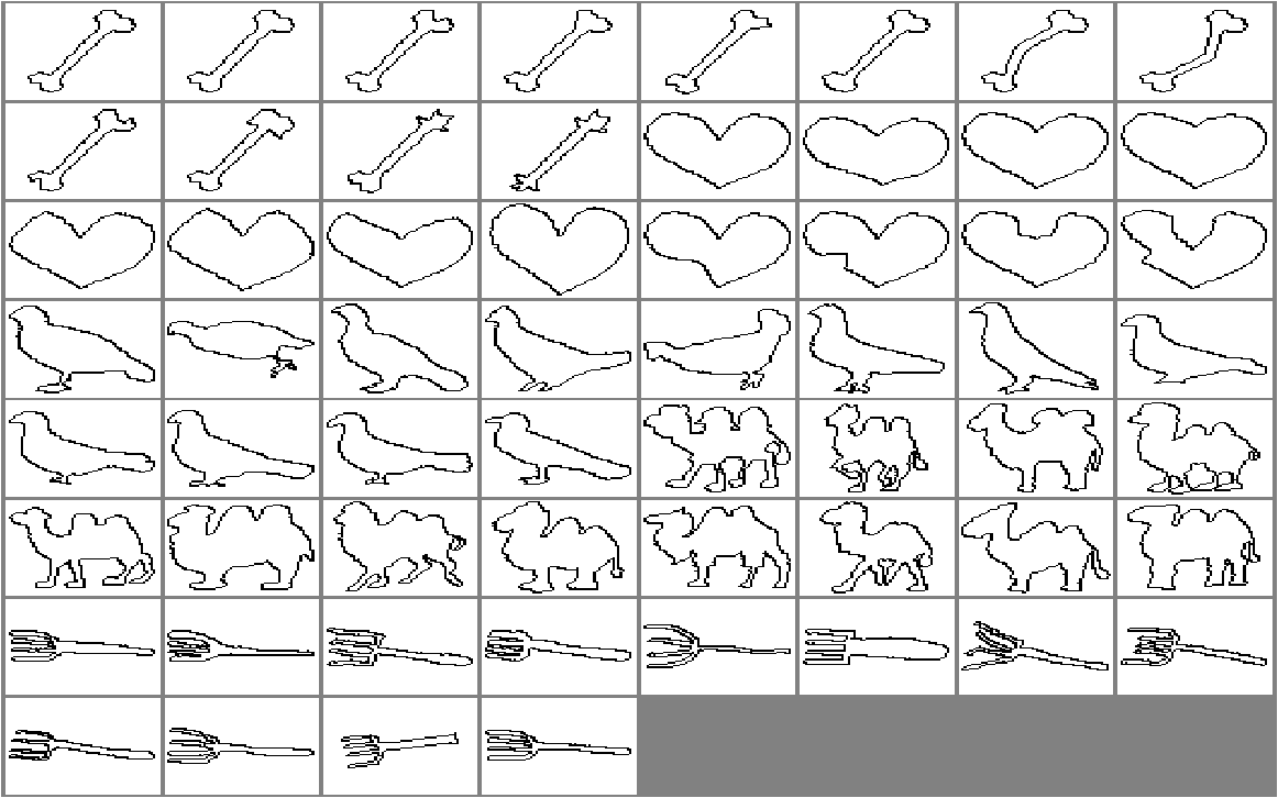
The perimeter can be estimated by a summation of all pixel values over an image.

    perimeter = im_stat(bor,'sum');

The two features, area and perimeter, are combined into a dataset which contains just these two values for every object. Some additional properties will be stored in the dataset as well: all classes are given the same prior probability (0.2, as there are 5 classes) and the names of the features.

    c = dataset([area perimeter]);
    c = setprior(c,0);
    c = setfeatlab(c,char('area','perimeter'));

This 2-dimensional dataset can be visualized

    figure; scatterd(c,'legend');

The name of the dataset is still known and shown in the figure. It was stored in the dataset a and transferred by PRTools to b, area and perimeter. The same holds for the class names, shown in the legend. Finally we will compute a classifier and show its decision boundary in the scatter plot. Different regions assigned to the various classes are given different colors.

    w = ldc(c);
    plotc(w,'col');
    showfigs

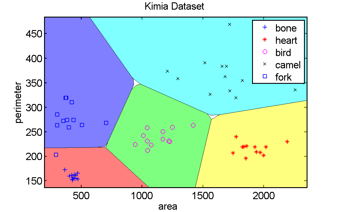
Note that there are some small regions that did not obtain a color. This is a numeric problem. Later it will be explained how to circumvent it. Can you identify the objects with almost no area and a large perimeter? And the objects with a relatively small perimeter and a large area? The scatter plot shows a representation based on features of the original objects, the silhouettes. It enables the training and usage of classifiers, which is an example of a generalization. The showfigs command distributes all figures over the screen in order to have a better display. Finally two classification errors are computed and displayed:

    train_error = c*w*testc;
    test_error = crossval(c,ldc,2);
    disp([train_error test_error])

The error in the training set, train_error, corresponds to the fraction of objects that are in the wrong class region in the scatter plot. The test error is estimated by 2-fold cross validation, a concept to be discussed later.

Example on silhouette classification