


 |
 |
 |
 | Image handling |
Images can be stored in datasets in different ways, depending on the interpretation of what objects and features are. They are handled by two commands, im2obj and im2feat. In order to understand the ways these commands work it has to be realized that images may be given by a set of bands (e.g. colors). In an N-band image every pixel is given by a vector of N elements. In a grey-value image N=1, in an RGB image N=3, for multiband images N > 3 and in hyperspectral images N might even be ar large as 1000.
Images can be stored in a dataset as object images or as feature images.
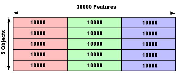
The entire image is considered as an object and its pixels as features. The dataset will then store a set of images. The feature size is the number of pixels. In case of a multiband image the bands are stored sequentially. So if 10 RGB images of size 256x256 are converted to a dataset, it has 10 objects with features of size 256*256*3. This is done such that first the red pixels, then the green and finally the blue pixels are stored. The feature size of a dataset storing such object images shows the size of the images in the featsize field, e.g. as [256 256 3].
In this case the images are not the objects but instead the pixel are the objects. They are given by the bands or the colors. So a single hyperspectral image of 256x256 pixels that consists of 1000 frequency bands is stored as a dataset of 256x256=65536 objects represented by 1000 features. In fact these are 1000 grey value images. The object size of a dataset storing such object images shows the size of the images in the objsize field, as [256 256] and in the featsize field as 1000.
Handling dataset images
In the below table the commands are listed that deal with the organization of images in datasets. Various types of operations for filtering or analyzing such images are discussed elsewhere.
| > Dataset image commands | |
| im2obj | The entire image is considered as an object and its pixels as features. The typical application is image recognition. The dataset will then store a set of images. The feature size is the number of pixels. In case of a multiband image the bands are stored sequentially. So if 10 RGB images of size 256x256 are converted to a dataset, it has 10 objects with features of size 256*256*3. This is done such that first the red pixels, then the green and finally the blue pixels are stored. |
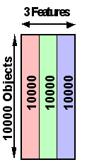
| im2feat | The pixels in an image are considered as objects. The features are the image bands. The typical application is image segmentation. A 256x256 RGB image has thereby 256x256 objects with 3 features. Usually just a single image is stored. If more images are stored the corresponding pixels are stored as additional objects. |
| obj2feat | Transform a dataset such that images stored as objects will be stored as features. |
| feat2obj | Transform a dataset such that images stored as features will be stored as object. |
| band2obj | Transform a dataset such that objects stored with multiple bands are split into sets of objects with a single band. |
| bandsel | Select image bands in dataset. |
| im_patch | Find / generate patches in dataset with images stored as objects. |
| data2im | Retrieves images stored in a dataset and reformats them appropriately. This is possible as the original images size is stored in the objsize and featsize fields of the dataset. This is of course not possible if the dataset has been sampled to retrieve an image. As soon as the image structure has been destroyed the image size information in these fields is lost. |
| show | Show the images as stored in a dataset. This makes use of the data2im command. |
Here it is symbolically illustrated how a set of RGB images is stored as objects in a dataset.
An example is the Kimia dataset that is stored in prdatasets.
    prdatasets; % checks or creates availability of prdatasets
    a = kimia   % load the datasets and display some information
%       Kimia Dataset, 216 by 4096 dataset with 18 classes: [12  12  12  12  12  12  12  12  12  12  12  12  12  12  12  12  12  12]

    struct(a)   % show the dataset fields
%        data: [216x4096 double]
%     lablist: {2x4 cell}
%        nlab: [216x1 double]
%     labtype: 'crisp'
%     targets: []
%     featlab: [4096x1 double]
%     featdom: {}
%       prior: []
%        cost: []
%     objsize: 216
%    featsize: [64 64]
%       ident: [1x1 struct]
%     version: {[1x1 struct]  '24-Mar-2011 23:06:09'}
%        name: 'Kimia Dataset'
%        user: []

    show(gendat(a,9) % show a random set of 9 images
Note that in the featsize field, [64 64], the image structure of the 4096 features (pixels) is stored.
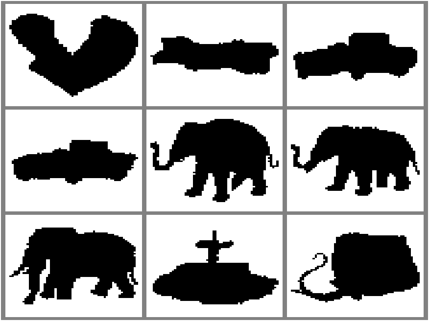
Note that the feature size is [64 64] as these are black-and-white images. Thereby they have just a single band, which has as a consequence that if the images are retrieved from the dataset the size shows
    im = data2im(a);
    size(im)
%       im =    64    64     1   216
that this is a set of 216 64x64x1 images.
Below a symbolic representation is shown of the way a single image is stored in a dataset by the im2feat command in which case pixels are the objects and the color bands are the features.
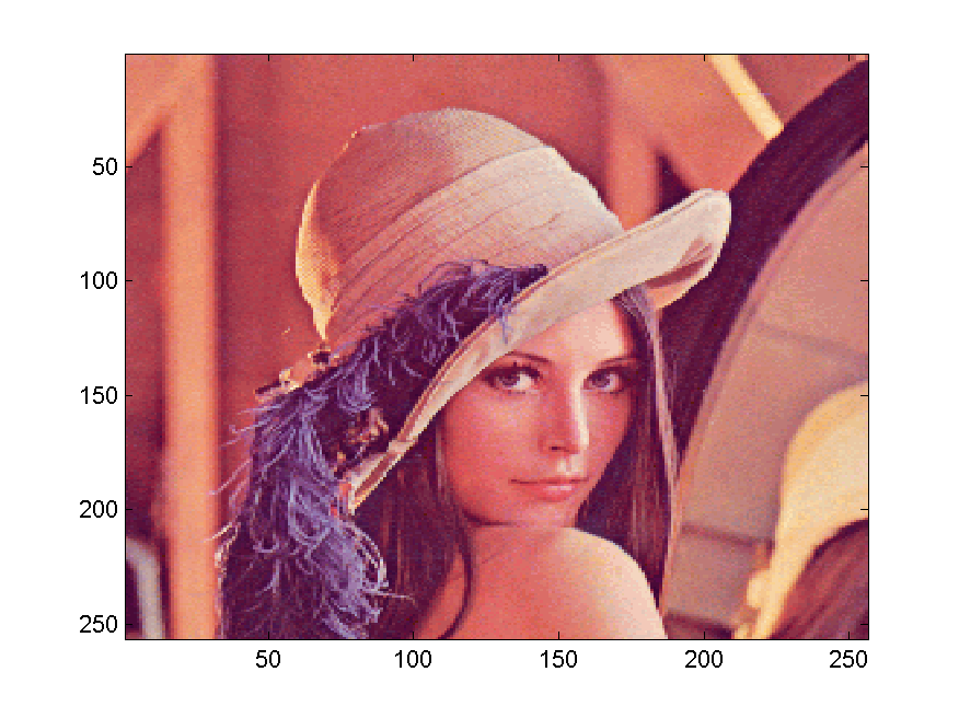
As an example we consider the famous Lena picture as it is stored in a dataset:
    a = lena
%       Lena, 65536 by 3 dataset with 1 class: [65536]

    struct(a)
%        data: [65536x3 double]
%     lablist: {2x4 cell}
%        nlab: [65536x1 double]
%     labtype: 'crisp'
%     targets: []
%     featlab: [3x5 char]
%     featdom: {}
%       prior: []
%        cost: []
%     objsize: [256 256]
%    featsize: 3
%       ident: [1x1 struct]
%     version: {[1x1 struct]  '24-Mar-2011 23:06:09'}
%        name: 'Lena'
%        user: []

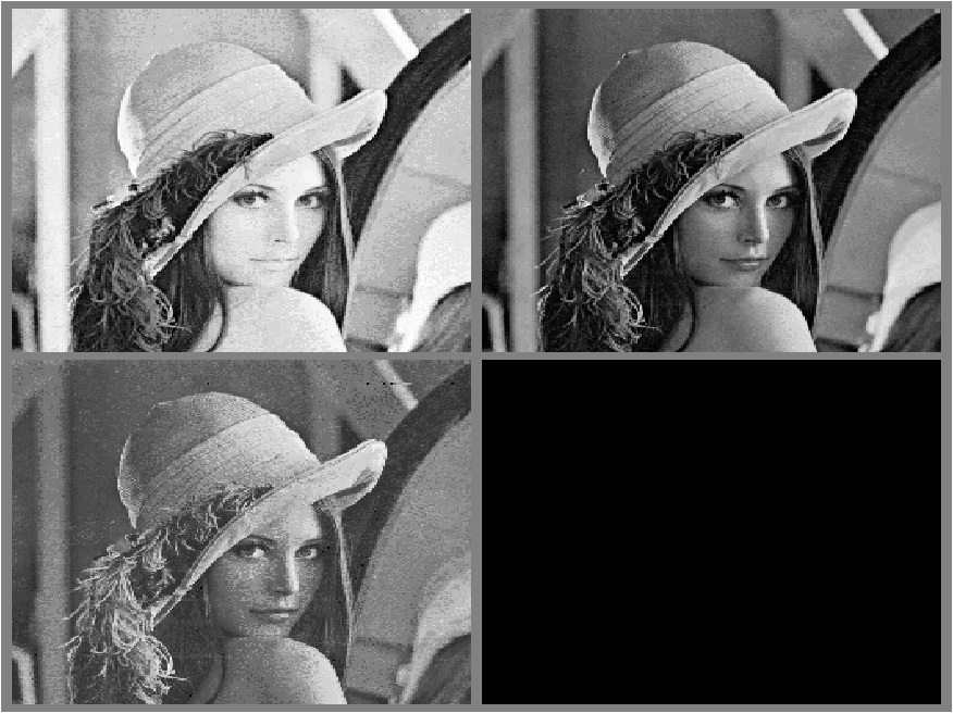
     show(a)

     image(data2im(a))
Note that in the objsize field the image structure, [256 256], of the 65536 objects, the pixels, is shown. The featsize is 3 as it is an RGB image. The show command displays every band separately in a sub-figure.
The original full color image can be displayed by the regular Matlab command image after the image is retrieved by data2im.
R.P.W. Duin
, January 28, 2013
 |
 |
 |
 | Image handling |